


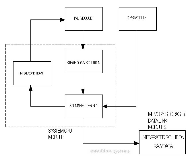
Waddan’s MAGI system provides a good example of system level software. In the system, the GPS and the IMU are two separate modules. The system CPU module computes the strapdown INS nav solution using the data received from the IMU. It also acquires the GPS nav solution from the GPS module. Then the CPU performs the Kalman filtering to integrate the two solutions to yield the GPS/INS integrated solution, as shown in the following block diagram.
Most of the MAGI system software is devoted to the Kalman filter for integrating the GPS/INS system. The system initialization passes through three mode–namely the Rough Leveling, the Coarse Alignment and the Fine Alignment. After the fine alignment, a reasonably accurate real-time integrated nav solution is obtained by employing a 15 state Kalman filter. The states of the filter are three components of position, velocity and attitude vectors; and three gyro biases and three accelerometer biases.
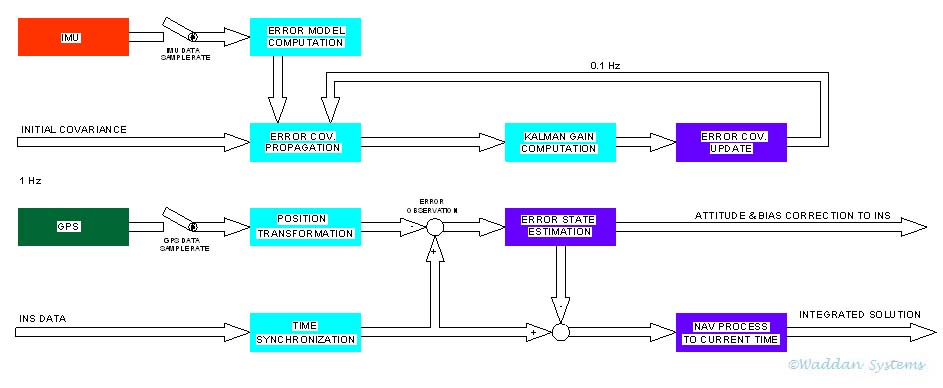
The block diagram above illustrates an approach for real-time implementation of the Kalman filtering. The computational steps leading to the integrated solution are:
Error Model Computation
An error model is a dynamic model in the state space to describe the propagation of the error sources in the navigation equations. A discrete system dynamic matrix is formulated to model the error states propagation. Since the dynamic matrix is a function of the vehicle maneuver, IMU data is required to generate this matrix. For the Fine Alignment, there are 15 states to be estimated. A 15 by 15 discrete system dynamic matrix is generated. Since the error states do not change fast, the data rate for computing the error model dynamic matrix is selected to be 1 Hz. The average of IMU data collected for one second is used to compute the error model dynamic matrix. This matrix is employed to propagate the error covariance matrix.
Error Covariance Propagation
An initial guessed error covariance matrix for the error states is used to propagate the covariance matrix using the discrete system dynamic matrix generated above. A process noise matrix derived from the AXLGYRO (sensor) noise characteristics is added to the covariance matrix. This matrix increases with time. As shown in block diagram, the error covariance matrix is processed every 1 Hz, which is the same as the error model computation update rate.
Kalman Gain Computation
The Kalman gain matrix is computed every time a GPS observation is made. The GPS observation made once every 10 seconds (i.e. at a rate of 0.1 Hz) is used for Kalman gain update computations. In reality, the gain update rate depends on the ratio of the process noise and the measurement noise of the system.
The GPS measurement noise is used for computing the error covariance matrix as well as the gain matrix. When no GPS data is available, the measurement noise is set to be infinite, thus making the corresponding Kalman gain matrix null. It means that no error states can be estimated in this case, and the integrated solution is same as the INS alone solution. Thus, the integrated solution is always better than or same as the INS alone solution.
Error Covariance Update
Once the Kalman gain matrix is computed and the corrections for the attitude and the biases for the INS sensors are completed, the error covariance matrix is updated. This updating process reduces the covariance error due to the observation. Thus, it is used in the next iteration of the error covariance propagation process as shown in the block diagram.
Position Transformation
The position and velocity obtained from the GPS receiver represent the position and the velocity at the GPS antenna. In order to compare the GPS data with that of the INS, the GPS antenna velocity and position must be transformed into the velocity and position at the IMU sensor location or vice-versa. Ignoring the structural compliances between these locations, the transformation would require the distance between their mounting locations, and the vehicle body attitude and rates.
Time Synchronization
Since the GPS data are available usually at 1 Hz frequency, and the INS data can be processed at 100 Hz or more; the velocity and position obtained from INS must be synchronized in time with the GPS data for a meaningful error observation. The GPS data time tag is used for the time synchronization. Any unprocessed IMU data is stored in the memory buffer for later processing.
Error State Estimation
The error observation is distributed to error states through Kalman gain matrix. This block in the above figure represents the computations of the optimal estimates of the error states. The error states include position errors, velocity errors, attitude errors, accelerometer bias errors and gyro bias errors. The resulting error state estimates are used for feedback to the INS navigation equations. This feedback process compensates the accelerometer and gyro biases, as well as correct the orientations of the sensor measurement axes in the strapdown navigation formulation.
Navigation Process to Current Time
Once the state errors are estimated using the observation error, the solution from INS is corrected by the estimated state errors. This corrected solution represent the best solution at the GPS observation time. Since the GPS data rate is l Hz , and the GPS observation can be late up to 1 second; additional navigation processing is necessary to compute the solution up to current time using the IMU data stored in the memory buffer.
